Advantages and Disadvantages of Random Forest in Modeling Species Distribution: From Theory to Practice
Species distribution model (SDM)
The concept of species distribution is deeply connected to the niche theory that begins to be formulated in the early 1900 (Johnson 1910; Grinnell 1917; Elton 1927) and was later innovated by Hutchinson in 1957. He first differentiated the niche into the fundamental and the realized one. The former measures the geographical area where the species can have a positive population growth considering all the abiotic factors, while the latter encompasses not only the abiotic effect but also the competition among species. Therefore, it made the realized niche smaller than the fundamental one. However, nowadays, we know that some biotic effects such as facilitation (positive interspecific interactions) can help the population positively to grow (Bruno et al. 2003). Since 2007, Soberon integrated the third critical factor, species dispersal or movement capacity, in the niche theory to consider if a species can reach a given area. He argued that before assessing if a particular species can thrive in the geographical area of interest where both abiotic and biotic conditions can satisfy the requirement of species, the species’ ability to arrive at that area must be examined. This is called biotic-abiotic-movement (BAM) concept that incorporates the interplay among these three factors into the assessment of species niche (Figure 1).

.
Figure 1. A BAM diagram suggests the three factors affecting the distribution of a species, abiotic factors (A), biotic factors (B), and dispersal or movement ability (M). It is adapted from Soberon (2007). The blue area between A and B indicates the area where the species can potentially have a positive growth considering its abiotic requirement and the prevailing biotic process, or also called “realized niche”. The intersection among A, B, and M (close circle area) represents the area where the species can move in and increase its population
Now, although we know that the SDM originated from the niche theory, the dispute still exists in which niche we are trying to study in SDM, is it the realized niche (the blue area in Figure 1), or the occupied niche (the close circle area in Figure 1), or none of both? There might not be a correct answer for now. Depend on the interest of research, the selected factors can be largely different, resulting in the distinctive niches measured. Indeed, according to the knowledge of the ecologist on the targeted species, the availability of abiotic data, and the sampling scale, the selection of predicting variables in SDM can be very different. Common climate data including in the models are often temperature, precipitation…etc. If your targeted species is the tropical scleractinian corals, factors other than those common ones such as light intensity and sedimentation should also be considered because of the reliance of corals on zooxanthellate. However, those two parameters are much less important in regulating the distribution of pelagic fish species which do not largely rely on light.
Common mathmatical approach used to fit and predict species distribution including profile techniques, group discriminative techniques, regression-based techniques, and machine learning. Profile techniques interprete the species distribution based only on the presence data, while the group discriminative techniques require not only presence but also absence data to generate SDMs. Example methods for the former is BIOCLIM (Busby 1991), and for the later is Maxent (Phillips et al. 2006). Regression-based techniques such as generalized linear model (GLM) and generalized additive model (GAM) look for the regression between the environmental factors and the species distribution. Lastly, machine learning can improve the performance by itself as it gets more and more data. For example, artificial neural networks (ANN) and random forest are ones of its algorithm.
Here, I would like to introduce the application of random forest on SDMs with a focus on the principle of Random forest, the advantages and disadvantages on the application, and a demonstration in R.
What is a random forest?
Random forest (RF) is a supervised learning algorithm that needs data to train. As its name, RF is an assemble of many individual decision trees which act as classifiers. Each tree can make a decision, and the final decision is made based on the mode (classification tree) or the average (regression tree) from all decision trees. It is commonly used to deal with classification, regression, or prediction tasks and also to measure the relative importance of the input variables. In addition, it is easy to use and the results it produces are usually good and quite straightforward. Combining all these features, it becomes one of the most popular algorithms in machine learning.
How does it work?
RF uses a bootstrapped procedure on the dataset to repeatedly create many subsets. Each of the subsets is later used to fit either a classification or a regression tree, and the final decision is made based on the mode or the average from those trees (Figure 2). Subsequently, an optimal model can be obtained by converging many classification and regression trees (CARTs) fitted by the bootstrapped samples. Based on this best model, we can predict the future observations. Here, I will explain step by step how does this algorithm work and terminology should be known to understand this algorithm.
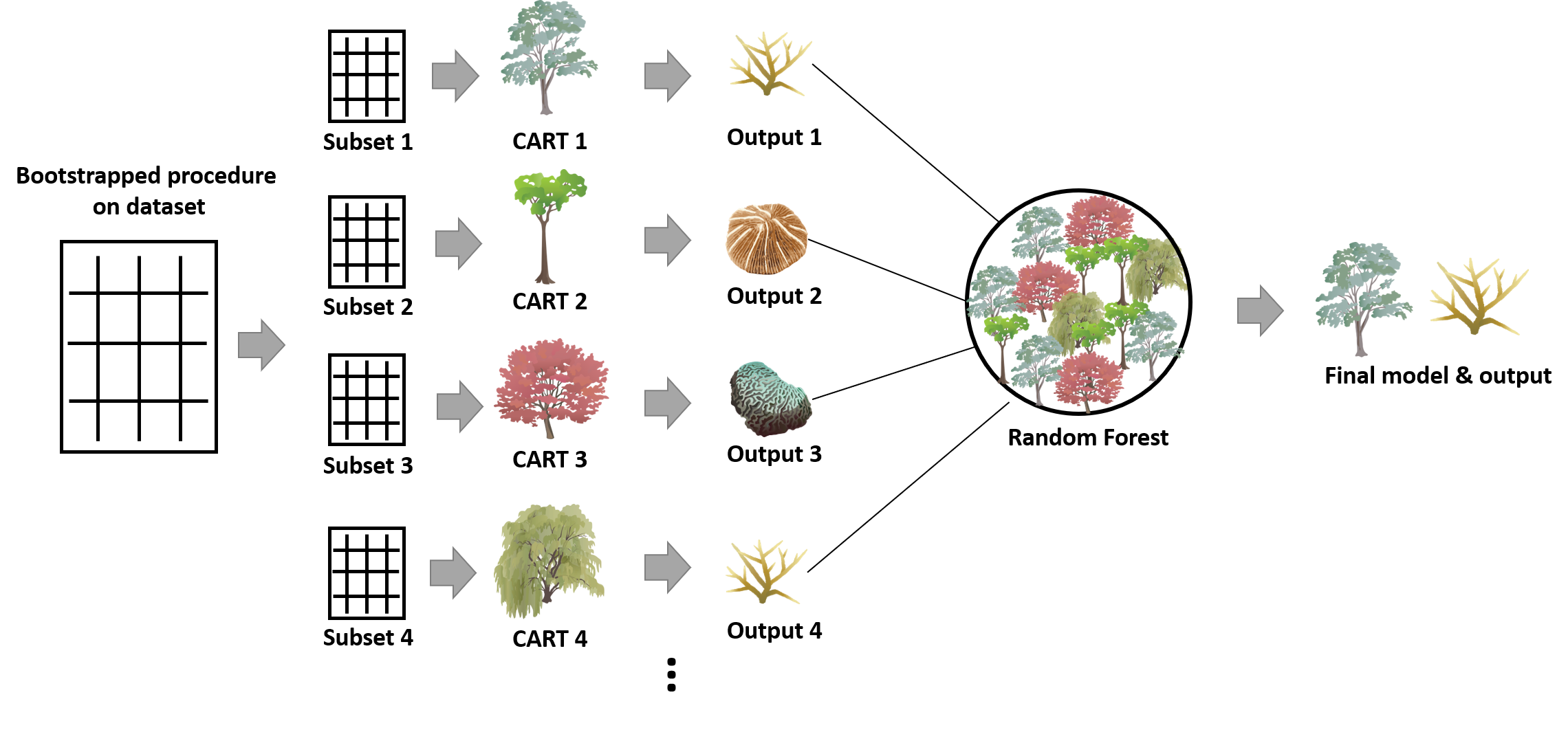
Figure 2. The framework of the RF algorithm
- Steps
Assuming I have a dataset (N) and the independent variables (M) that I think are important features to delineate those observations. By applying RF to this dataset, I can (1) find out the best model to fit this dataset, (2) predict the future observations according to this model, and (3) calculate the importance of those feature variables. These three tasks are very helpful for solving the research questions regarding to SDM, and that is probably why RF is attractive to these users. The procedure of this algorithm is:
- Build n bootstrap replicates from the dataset N with the equal sampling size (with replacement). For each replicate, a tree will be created. In other words, n is also the number of trees to fit.
- Divide each bootstrap replicate into a training and a testing set. The ratio of data in two sets can be 9:1, 8:2, 7:3, or any ratio, there is no fixed rule. It depends on if the performance of the final model meet your expectation or not.
- For each replicate, fit a tree to the training set. At each node of the tree, a permutation procedure randomly selecting m feature variables from the variable set (M) is conducted to find out the best split based on the Gini Index (see below) that can quantify the within-node entropy. After this tree is successfully made, it would be validated with the testing set. The prediction error of the classification tree is measured by out-of-bag (bootstrapping) error while the one of the regression tree is calculated by mean squared error.
- Asemble n trees to find out the best model.
- Based on this model, a prediction can be made for the future observations.
- Classification and regression tree (CART)
CART is a classifier used to sort the observations based on recursive binary decisions. These decisions are made by the given feature variables which have the most information. However, how does the CART decide the binary decisions on each split? Before answering it, we have to know what is a Gini Index. Gini Index can measure the probability of a specific variable being incorrectly classified when randomly selected. This index is entropy-based, so their interpretation is similar. Gini Index ranges between 0 to 1, while 0 denotes that all the elements belong to a single class or there is only one class existing (pure), 1 denotes that all the elements randomly distribute among the classes (impure). Mathematically, it is expressed as:
\[ Gini Index=1-\sum_{i = 1}^{n}{(p_i)^2} \] where pi denotes the probability of an element being classified to a specific class.
In each split of a tree, Gini Indeces for each of the variables randomly picked up from its variable set are calculated, and the one with the lowest Gini Index is chosen as the given split (Figure 3). For the part of variables, the more a variable contributes to the prediction process, the more chances it would be retained as the split. While for the observation, the more binary decisions the CART makes, the more similar the feature variables of the subset groups (Figure 3). Nonetheless, more splits on a tree do not necessarily make the model perform better, too many splits may lead to the overfitting of the model.
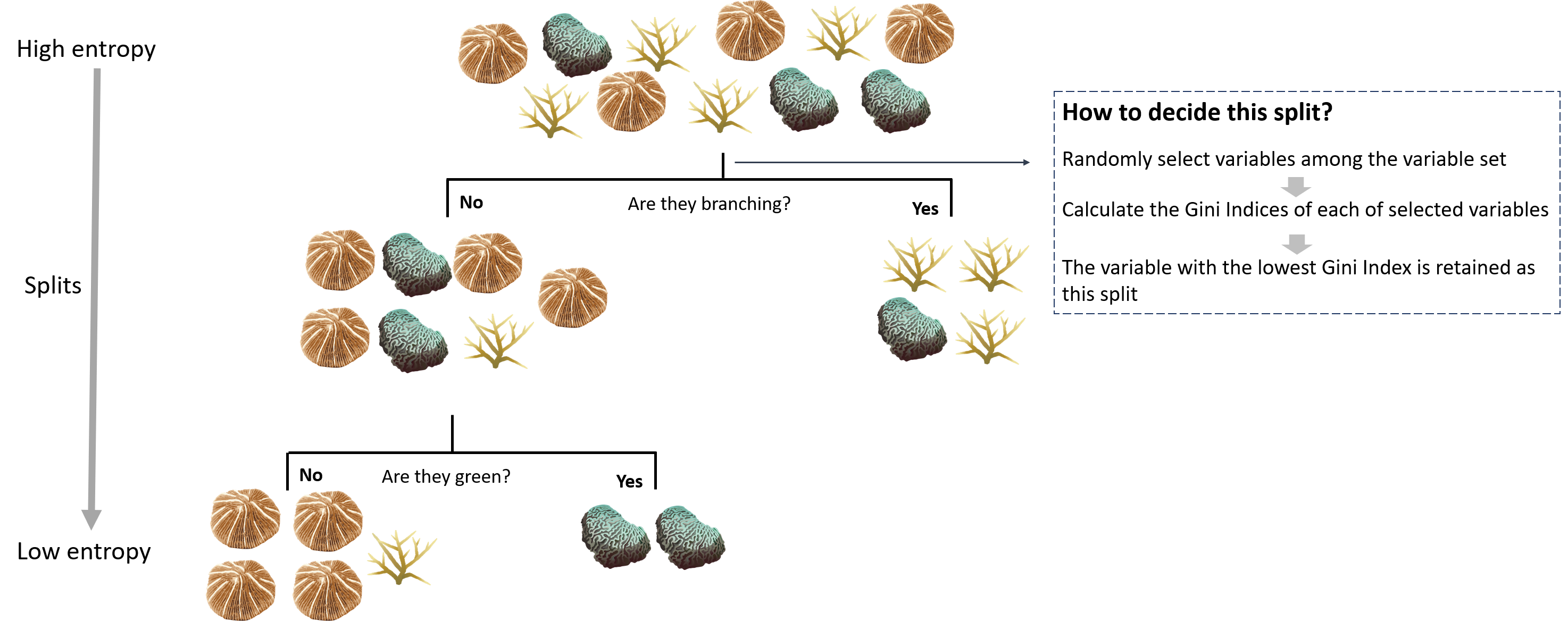
Figure 3. A CART trying to classify corals based on their morphology and color. The entropy of the dataset decreases each time a split is made.
- Variable importance
An excellent piece of information that we can derive from RF is the relative importance of each feature variable on the predictions.
There are two kinds of measures. The first one measures the mean decrease in the accuracy. It measures the loss of accuracy when excluding the particular variable from the prediction model. Specifically, for each tree, the out-of-bag error (or mean squared error for the regression tree) is computed from its testing data. Then, the error is calculated again after permuting the values of each feature variable in testing data. The difference between the two error values is later averaged over all the trees. After normalization, the value obtained is the decrease in prediction accuracy.
The second measure is based on the decrease in Gini Index when a variable is selected as a split. In particular, it calculates for each variable the sum of the decrease in the Gini Index from each tree when it is chosen as the split. Then, this sum is divided by the total number of trees built to gain the decrease in the Gini Index of that variable.
- Hyperparameter tuning
Hyperparameter tuning refers to a set of parameters that needs to be decided before starting the algorithm. Those parameters can be adjusted either to make the model perform better or to fasten the model. These are some common parameters that can be set before conducting the RF in R (function: randomforest).
Number of trees (ntree)
Number of feature variables randomly sampled as candidates at each split. (mtry)
There are still many hyperparameters that you cna adjust (eg. size(s) of sample to draw), however, I so not introduce them since they are less used. Check more information about this here.
Advantages and disadvantages
After understanding both SDM and RF, we can start to talk about why RF becomes more and more popular in fitting SDM recently. It has several advantages when combining both:
No need for assumptions before conducting the models (e.g. independence of variables, normal distribution). This is a very great asset of this non-parametric model, which makes it outcompete other linear-based models (e.g. generalized linear model). One of the required assumptions before conducting the traditional linear-based models is the independence of variables. However, some environmental data are naturally spatially or temporally autocorrelated, additional statistical steps have to be implemented to deal with this issue before starting the linear-based models. Another required assumption when building linear-based models is the normality, however, these environmental data are usually not normally distributed. In this condition, RF is a non-parametric model that can still work when the normality of the data is not meet.
Flexibility to address several types of analysis. As mentioned earlier, RF can address many kinds of statistical analyses or models such as regression, classification, prediction. This flexibility makes RF very useful in modeling species distribution. For example, common types of environmental predictors include categorical and continuous, and the species data can be either presence-absence or abundance. The good news is, RF is able to integrate all of them.
Identify non-linear relationships. The response of species to the environmental condition or change is not always linear, it can be exponential, concave…etc. Sometimes, these non-linear interactions between the environmental factors and species can also be meaningful to affect species distribution. The advantage of RF is that it can uncover non-linear relationships that the linear-based models cannot find. In addition, another limitation when using the linear-based model to fit SDMs is that those linear-based models can only test a priori hypothesis and are, therefore, hard to detect the relationship out of this expectation. On the other hand, RF is also able to figure out the complex interactions between environmental variables. For example, they may interact hierarchically with each other. This is because the RF is an assemble of many CARTs, so it can address the environmental factors that interact with hierarchy.
Allowing missing value. The RF automatically produces proximity, which is the measure of similarity among data points. This proximity matrix can be used to simulate the missing data that could be obtained when ecologists have to simultaneously sample species and environmental data.
Less overfitting. The RF tends to be less overfitting than the CART. CART sometimes overfits the data because it would continuously split the nodes to minimize the within-node entropy. However, this issue is overcome in RF by choosing the best CART from many of them through the out-of-bag procedure/averaging many CARTs and also by randomly selecting the candidate variables in each node of trees. Overfitting is the last issue we would like to encounter when constructing a model since it could make the model perform badly in prediction, so does the SDM.
It seems it is perfect to model the distribution of species with RF. Nonetheless, several disadvantages still exist when conducting it:
Blackbox approach. The ecologists have very few controls on what the algorithm does, basically, they can only try with different settings of hyperparameters (see the section of hyperparameter tuning) and different ratios of training and testing sets, then check the model afterward. This blackbox effect can sometimes make the results hard to interpret, however, this may not be a big issue if the ecologists already have a basic understanding of the species they are working on.
A large number of trees make the algorithm slow to run. A large enough dataset, as well as number of trees, has to be prepared and built to gain a robust RF model. This process can make the algorithm time-consuming. However, this step is important to avoid the overfitting issue that may occur for the CART mentioned earlier (Point 5 in Advantage). Therefore, the users have to deal with this trade-off between the time running for the RF model and its performance.
Demonstration in R
Background
To demonstrate how to apply RF on SDM in R, I chose three abiotic factors, sea surface temperature (SST), light at the surveyed depth, and chlorophyll a, to model the distribution of a scleractinian coral species, Stylophora pistillata. The cover data of the coral species from 209 transects sampled in the north, east, and south Taiwan during 2015-2020 were derived from my Ph.D. research project. Each transect sampled a 5.25m2 area and one unit value in species cover represent the area among 5.25 m2. As for the three abiotic parameters, I computed their 2014 mean annual values averaging the 12 months data downloaded from the ERDDP server managed by National Oceanic and Atmospheric Administration (NOAA), USA (dataset ID for temperature is NOAA_DHW, for chlorophyll a is erdMH1chlamday, for light at the surveyed depth are erdMH1par0mday and erdMH1kd490mday1). Since the abiotic variables I chose are all continuous ones, I will demonstrate the RF with regression trees instead of classification ones.
1 light at the surveyed depth = PAR x exp (-kd490 x z) where PAR is photosynthetically available radiation, kd49 means diffuse attenuation k490, and z represents the in situ depth.
Download the data
Before starting the analysis, you can download the the datasets (cover of S. pistillata and abiotic factors in the sampling sites, the abiotic factors around Taiwan, coordinates of sampling transects, the three map files of Taiwan), and the R manuscript to follow this RF analysis.
Download Stylophora_pistillata.xlsxDownload env.csv
Download cord.xlsx
Download TWN_adm0.shp
Download TWN_adm0.dbf
Download TWN_adm0.shx
Download index.R
Start the analysis
Package installation
# install.packages(c('readxl','randomForest','rgdal','ggplot2','sf','tmap','sp'))
# update.packages()
library(readxl)
library(randomForest)
library(rgdal)
library(ggplot2)
library(sf)
library(tmap)
library(sp)
Data importation
# setwd('') # set your local path
stpi.data <- read_excel("Stylophora_pistillata.xlsx") # import Stylophora pistillata cover and environmental data from 209 transects
stpi <- stpi.data[ ,-c(1,2)] # remove the column with transect information
cord <- read_excel("cord.xlsx") # import the coordinate of sampling transects
taiwan <- readOGR('TWN_adm0.shp') # import the OGR file of Taiwan map
pred.env <- read.csv("env.csv") # import the coordinate of sampling transects
pred.env <- pred.env[,-1]
After importing all the files, let’s start to build the species distribution model with RF.
Model construction
Then, I can start to create the model.
set.seed(1) # set a random seed to make the model reproducible
rf.stpi <- randomForest(SP ~ .,data=stpi, importance = T) # build the random forest model
rf.stpi
##
## Call:
## randomForest(formula = SP ~ ., data = stpi, importance = T)
## Type of random forest: regression
## Number of trees: 500
## No. of variables tried at each split: 1
##
## Mean of squared residuals: 0.001531159
## % Var explained: 25.43The result of this model shows that the three factors can together explain 25.43% of the total variance. This is not high, but with only three variables, it is also not bad. Still, more abiotic factors are recommended to add to this model to catch more variance. I use 500 trees (R’s default) to build this model, and caution is needed for the number of trees since too many trees may make the model overfitting. Therefore, checking the mean square errors of models created with the different number of trees is recommended.
Notice: despite we use the same dataset, the RF models generated each time would be slightly different from the ones here. This is normal because the RF contains the bootstrapping process making the trees constructed each time are different. However, we would like our analyses to be reproducible, the function “set.seed” is then useful here. You can use this function to fix the outcome as long as you fill in the same number each time you produce the model so that the result would be reproducible. As such, the result you get may be different from this demonstration.
plot(rf.stpi) # check the mean square error of models
From the plot, we know that as more and more trees are built, the errors decrease and eventually become stable. It seems that when the number of trees is around 10-100, we arrived at the lowest error. We can check it with the “which.min” function.
which.min(rf.stpi$mse)## [1] 49It turns out that we can have the lowest error in the RF model with 49 trees, so let’s rebuild the model with this number of trees by using the argument “ntree”.
Then, I can start to create the model.
rf.stpi.min <- randomForest(SP ~ ., data=stpi, importance = T, ntree=49)
rf.stpi.min
##
## Call:
## randomForest(formula = SP ~ ., data = stpi, importance = T, ntree = 49)
## Type of random forest: regression
## Number of trees: 49
## No. of variables tried at each split: 1
##
## Mean of squared residuals: 0.001518843
## % Var explained: 26.03The variance explained slightly increase and the error slightly decrease, so this model performs a little bit better than the one with 500 trees. In addition to this hyperparameter, we can also adjust the number of the variables randomly selected at each split with the argument “mtry” to make the model perform better.
rf.stpi.min.2 <- randomForest(SP ~ ., data=stpi, importance = T, ntree=49, mtry=2)
rf.stpi.min.2
##
## Call:
## randomForest(formula = SP ~ ., data = stpi, importance = T, ntree = 49, mtry = 2)
## Type of random forest: regression
## Number of trees: 49
## No. of variables tried at each split: 2
##
## Mean of squared residuals: 0.001536821
## % Var explained: 25.16rf.stpi.min.3 <- randomForest(SP ~ ., data=stpi, importance = T, ntree=49, mtry=3)
rf.stpi.min.3##
## Call:
## randomForest(formula = SP ~ ., data = stpi, importance = T, ntree = 49, mtry = 3)
## Type of random forest: regression
## Number of trees: 49
## No. of variables tried at each split: 3
##
## Mean of squared residuals: 0.001581607
## % Var explained: 22.97
The models with 1 variables tried at each split does the best since it has the minimum error. The variance explained also increase a bit. Hence, we will use the one with mtry = 1.
To split the whole dataset into training and testing set in RF?
Some people may argue to split the whole dataset into training and testing set before conducting the RF so that the model can be validated later on. However, it is not an obligation to do so since when conducting the randomforest function in R, it already bootstraps the whole dataset and further classify each replicate into training and testing set, then fit a tree with the training set. In other word, each observation would be excluded for multiple time when building the trees during this bootstrapping process. The total error of this model (out-of-bag error or mean squared error) is then computed by averaging all the errors calculated based on each observation. Therefore, based on this process, the error itself is already able to represent the validation error. However, depends on your dataset and purpose, you can still split the dataset and do the cross-validation. People may do so in the following situations:
Big dataset. When your dataset is big enough, it can allow you to robustly validate your model with the testing set (that is why I do not demonstrate this part because the dataset we use here is relatively small).
Optimize the hyperparameters. You can determine your hyperparameters based on the training set you get after splitting, and check the performance of the hyperparameters using the remaining testing set. It is always good to test your hyperparameter setting with the unused dataset to have an unbiased estimation.
Compare the RF performance to other models. In this case, you may keep a testing set so that can allow you to validate different models with the same data to make a fair comparison.
Performance of the model
Now, we can check the performance of this model by calculating the residuals and the mean squared error. We first use the whole dataset to run the prediction of this model and check the difference between the observed and the predicted values, which is the residuals.
pred.stpi <- predict(rf.stpi.min, newdata=stpi)
rf.resid.stpi <- pred.stpi - stpi$SP # the residuals
plot(stpi$SP,rf.resid.stpi, pch=18,ylab="residuals (predicted-observed)",   xlab="observed",col="blue3") # residual plot
abline(h=0,col="red4",lty=2)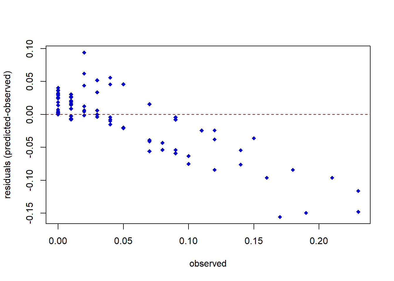
The residual plot shows that the error of the model is around 0-10% when predicting the distribution of S. pistillata, and more error would be found in the area with higher cover. This may be because there are too little data especially in the geographical area with the higher cover of S. pistillata.
Then, let’s check the mean squared error of this model.
mean(rf.resid.stpi^2) # mean squared error## [1] 0.001077198This value alone might not be able to tell us the quality of this model. However, it is important when we would like to compare this RF model to other ones (eg. GLMs). We can use this mean squared error to make a comparision, the lower it is, the better it is. Eventually, we can figure out the best model.
Prediction
After selecting the best hyperparameter setting and check its performance, we can start to use this model to predict. In this case, the first question comes to our mind may be the prediction of coral cover on the areas where we do not sample. Therefore, I extract the 0.1 x 0.1 degree grid data of three environmental factors around Taiwan (latitude: 20-26°N, longitude: 115-125 °E), and would like to predict the cover of S. pistillata with these factors. To make the result easier to compart and more visualize, I make the prediction by depths.
pred.env.5 <- data.frame(pred.env$light.5,pred.env$SST,pred.env$chl)
colnames(pred.env.5) <- c('light','Chl_a','SST')
pred.5 <- predict(rf.stpi.min, newdata=pred.env.5)
pred.env.10 <- data.frame(pred.env$light.10,pred.env$SST,pred.env$chl)
colnames(pred.env.10) <- c('light','Chl_a','SST')
pred.10 <- predict(rf.stpi.min, newdata=pred.env.10)
pred.env.15 <- data.frame(pred.env$light.15,pred.env$SST,pred.env$chl)
colnames(pred.env.15) <- c('light','Chl_a','SST')
pred.15 <- predict(rf.stpi.min, newdata=pred.env.15)
pred.env.40 <- data.frame(pred.env$light.40,pred.env$SST,pred.env$chl)
colnames(pred.env.40) <- c('light','Chl_a','SST')
pred.40 <- predict(rf.stpi.min, newdata=pred.env.40)
summary(pred.5)
## Min. 1st Qu. Median Mean 3rd Qu. Max. NA's
## 0.0526 0.0692 0.0692 0.0705 0.0692 0.0897 2274summary(pred.10)## Min. 1st Qu. Median Mean 3rd Qu. Max. NA's
## 0.0211 0.0692 0.0692 0.0668 0.0710 0.0897 2274summary(pred.15)## Min. 1st Qu. Median Mean 3rd Qu. Max. NA's
## 0.0211 0.0574 0.0720 0.0614 0.0733 0.0897 2274summary(pred.40)## Min. 1st Qu. Median Mean 3rd Qu. Max. NA's
## 0.0211 0.0211 0.0240 0.0268 0.0260 0.0526 2274According to the outcome, the predicted coral covers decrease as the depths increase. The maximum and the minimum covers also follow this pattern. There are also many missing values (2274 among 2700 observations), the common way to solve this issue is to either take the environmental value of the adjacent grids or calculate the average from the adjacent grids to represent the value in the grid with missing value.
Variable importance
In addition to the prediction, the other information that people may try to get from this RF model is the variable importance. This information can also help us better explain the predicted pattern we just obtain. Now, we can check the importance of those variables in this model with the function “varImpPlot” and ”importance”.
varImpPlot(rf.stpi.min)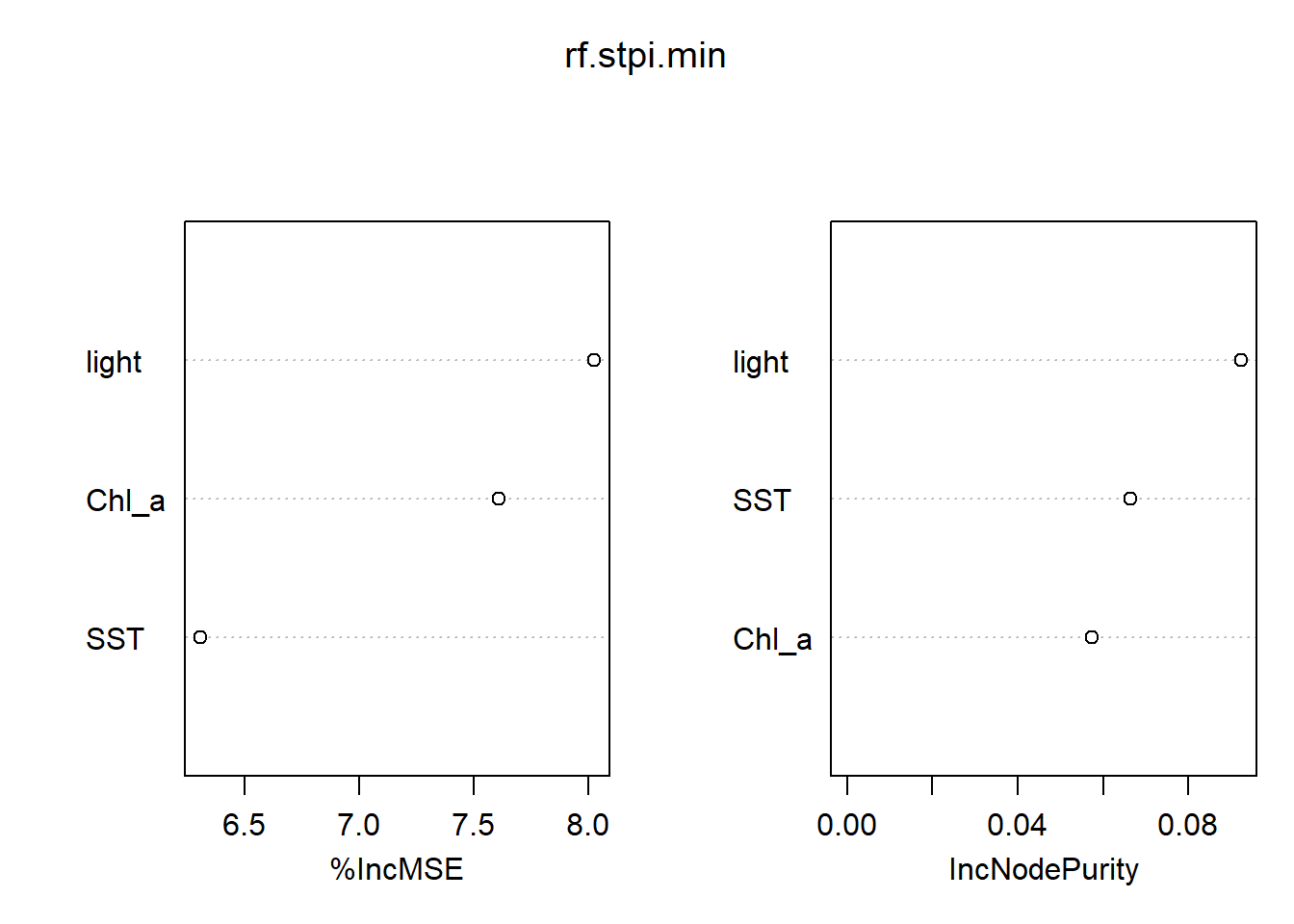
importance(rf.stpi.min)## %IncMSE IncNodePurity
## light 8.025663 0.09225743
## SST 6.306275 0.06631249
## Chl_a 7.611486 0.05732706The result shows the importance of variables calculated with the mean decrease in accuracy and with the Gini Index. Both suggest that light is the most important factor in driving the distribution of S. pistillata. However, the former shows that the chlorophyll a is the second important variable followed by SST while the later suggests the reverse for these two factors.
The effect of abiotic factors on the coral cover prediction
Then, we can have a look on how the individual abiotic variable affecting the model with partial plots with the function ”partialPlot”.
par(mfrow=c(1,3))
partialPlot(rf.stpi.min, as.data.frame(stpi), light)
partialPlot(rf.stpi.min, as.data.frame(stpi), SST)
partialPlot(rf.stpi.min, as.data.frame(stpi), Chl_a)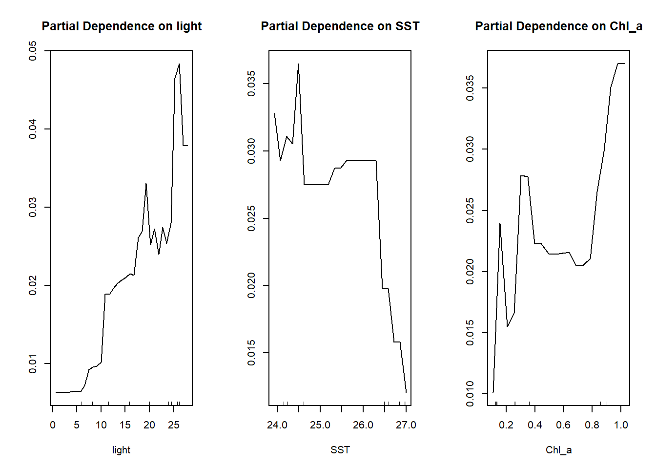
dev.off()The purpose of the partial plot is to display how the prediction of coral cover is changing with the change of each of the three abiotic variables. If the line is closer to zero, it means that the given variable is not affecting the coral cover at all, while the more the line deviating from zero, this variable influences the coral cover more. For example, from the three plots above, we can tell that the light has more influence on the prediction of the coral cover than the other two factors.
Instead of looking at the value on the y-axis, the relationship between the y-axis and the given variable across a specific range is what we should focus on. For example, in the partial dependence plot on light, when the light intensity becomes stronger we have more chances to see a high cover of S. pistillata. This increase of chances is even more obvious when the light intensity is between 5 to 15 W/m2/day and over 25 W/m2/day. Look at the partial dependence plot on SST, we found that the cover of S. pistillata would dramatically decrease when the 2014 mean SST is above 26 °C and its cover remains quite consistent when it is below 26 °C. Lastly, for the partial dependence plot on chlorophyll a, it peaks when the concentration of chlorophyll a is at around 0.2, 0.4, and 1 mg/m3. By checking the tendency and the value in the y-axis on these three partial plots, it could explain why light intensity is the most important factor in predicting the distribution of S. pistillata.
Species distribution map (observed and predicted)
Now, let’s also draw the distribution map of S. pistillata with observed and predicted cover information to visualize it. Since I would like to use a grid map with 0.1 x 0.1 degree resolution to visualize it (same than the resolution of environmental factors used in the prediction), I have to figure out which grids my sampling sites locate in. Consequently, I write a function to figure out which grids my sampling sites locate in and the observed and predicted coral cover in these grids, and also average the cover of transects if the number of the transects in one grid is more than one. In this function, I can specify the coordinate matrix (with coordinate, depth, observed, predicted coral cover information), the depths and the grid resolution (degree) I would like to use. The outcomes of this function contain three data frames with the information about 1) the grids my sampling sites locate in, 2) the summary of the observed and predicted coral cover in each grid, and 3) the observed and predicted coral cover in each grid (1 means there is no cover data). Then, I use the outcome of this function to make the observed and predicted maps in my sampling sites with the “tmap” package in R.
taiwan.sf <- st_as_sf(taiwan) # tranform the sp file to sf file
cord.all <- cbind(cord, stpi.data, pred.stpi) # create a matrix with coordinate, observed, predicted cover for the sampling sites
# creat a function to match the sampling sites and the grid system I created
# I can specify the matix (with coordinate, depth, observed, predicted coral cover
# information), the depths and the grid resolution (degree) I would like to use
grid.match.depth <- function(matrix, depth, resolution){
  cover <- subset(matrix , Depth==depth) # subset the matrix with the depth
  lat <- as.factor(cover$Lat) # setup the latitude as factor
  lon <- as.factor(cover$Lon) # setup the longitude as factor
  coords <- SpatialPoints(cover[, c("Lon", "Lat")]) # transfer the latitude & longitude into spatialpoint (for map)
  proj4string(coords) <- '+proj=longlat +datum=WGS84 +no_defs' # assign the coordinate projection system to the same one with the Taiwanese map

  # creat a grid system
  bb <- bbox(taiwan) # set up the boundary of this system to the same with the Taiwanese map
  cs <- c(1, 1)*resolution  # cell size (degree) : using the argument "resolution" to specify
  cc <- bb[, 1] + (cs/2)  # cell offset
  cd <- ceiling(diff(t(bb))/cs)  # number of cells per direction
  grd <- GridTopology(cellcentre.offset=cc, cellsize=cs, cells.dim=cd) # cell topology
  sp_grd <- SpatialGridDataFrame(grd, data=data.frame(id=1:prod(cd)), proj4string='+proj=longlat +datum=WGS84 +no_defs') # create a sp data frame

  grid.over <- cbind(over(coords, sp_grd),cover$SP ,cover$pred.stpi) # create a matrix with observed coral cover & predicted cover
  colnames(grid.over) <- c('id','obs.cover','pred.cover') # remane the matrix
  grid.over.mean <- aggregate(obs.cover~id, grid.over,mean) # at least 5 transects sampled in the same grid, average the observed cover of those transects
  loc <- as.numeric(grid.over.mean$id) # setup the id of the grids as numerical
  id <- rep(1, prod(cd)) # setup a id vector with 1
  over <- replace(id,loc,grid.over.mean$obs.cover) # replace the ids with coral cover information with the mean observed coral cover
  grid.over.mean.pred <- aggregate(pred.cover~id, grid.over,mean) # at least 5 transects sampled in the same grid, average the predicted cover of those transects
  loc.pred <- as.numeric(grid.over.mean.pred$id) # setup the id of the grids as numerical
  id.pred <- rep(1, prod(cd)) # setup a id vector with 1
  over.pred <- replace(id.pred,loc.pred,grid.over.mean.pred$pred.cover) # replace the ids with coral cover information with the mean predicted coral cover
  sp.grd <- SpatialGridDataFrame(grd,data=data.frame(observed.cover = over, predicted.cover = over.pred), # create a spatial data frame with the observed and predicted cover
                                 proj4string='+proj=longlat +datum=WGS84 +no_defs')

  return(list(grid.over,summary(sp.grd),sp.grd)) # return the result
}
layer.5m <- grid.match.depth(cord.all,5,0.1) # extract the information of 5m
sp.grd.5 <- layer.5m[[3]][1] # assign the 5m observed cover to the matrix
sp.grd.5.pred <- layer.5m[[3]][2] # assign the 5m predicted cover to the matrix
layer.10m <- grid.match.depth(cord.all,10,0.1)  # extract the information of 10m
sp.grd.10 <- layer.10m[[3]][1] # assign the 10m observed cover to the matrix
sp.grd.10.pred <- layer.10m[[3]][2] # assign the 10m predicted cover to the matrix
layer.15m <- grid.match.depth(cord.all,15,0.1)  # extract the information of 15m
sp.grd.15 <- layer.15m[[3]][1] # assign the 15m observed cover to the matrix
sp.grd.15.pred <- layer.15m[[3]][2] # assign the 15m predicted cover to the matrix
layer.40m <- grid.match.depth(cord.all,40,0.1)  # extract the information of 40m
sp.grd.40 <- layer.40m[[3]][1] # assign the 40m observed cover to the matrix
sp.grd.40.pred <- layer.40m[[3]][2] # assign the 40m predicted cover to the matrix
bb <- bbox(taiwan) # set up the boundary of this system to the same with the Taiwanese map
cs <- c(1, 1)*0.1  # cell size 0.1 x 0.1 degree
cc <- bb[, 1] + (cs/2)  # cell offset
cd <- ceiling(diff(t(bb))/cs)  # number of cells per direction
grd <- GridTopology(cellcentre.offset=cc, cellsize=cs, cells.dim=cd) # cell topology
sp_grd <- SpatialGridDataFrame(grd,data=data.frame(id=1:prod(cd)), proj4string='+proj=longlat +datum=WGS84 +no_defs')
sp.grd.all <- SpatialGridDataFrame(grd,data=data.frame(coral.cover.5m = sp.grd.5$observed.cover, # create a spatial data frame with the observed cover for mapping
                                                       coral.cover.10m = sp.grd.10$observed.cover,
                                                       coral.cover.15m = sp.grd.15$observed.cover,
                                                       coral.cover.40m = sp.grd.40$observed.cover),
                                   proj4string='+proj=longlat +datum=WGS84 +no_defs')
sp.grd.all.sf <- st_as_sf(sp.grd.all) # tranform the sp file to the sf file
sp.grd.pred.all <- SpatialGridDataFrame(grd,data=data.frame(coral.cover.5m = sp.grd.5.pred$predicted.cover, # create a spatial data frame with the predicted cover in sampling sites for mapping
                                                            coral.cover.10m = sp.grd.10.pred$predicted.cover,
                                                            coral.cover.15m = sp.grd.15.pred$predicted.cover,
                                                            coral.cover.40m = sp.grd.40.pred$predicted.cover),
                                        proj4string='+proj=longlat +datum=WGS84 +no_defs')
sp.grd.all.pred.sf <- st_as_sf(sp.grd.pred.all) # tranform the sp file to the sf file
# draw the maps
col.pan <- c("lightblue","blue","green", "yellow","orange","red","white") # setup the color panel for mapping the cover
tmap_mode("plot")
tm_shape(sp.grd.all.sf) +
  tm_symbols(c("coral.cover.5m","coral.cover.10m","coral.cover.15m","coral.cover.40m"),
             size=1,breaks = c(seq(0,0.12,0.02),1),shape=15,
             palette = col.pan, title.size = 2, border.col =NA,
             labels = c("0-0.02", "0.02-0.04", "0.04-0.06","0.06-0.08","0.08-0.10","0.10-0.12","No cover data"))+
tm_shape(taiwan.sf) +
  tm_polygons("Islands",legend.show = F, alpha =.3,)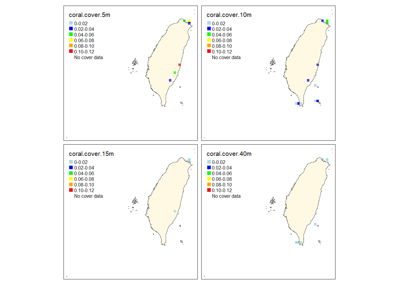
tm_shape(sp.grd.all.pred.sf) +
  tm_symbols(c("coral.cover.5m","coral.cover.10m","coral.cover.15m","coral.cover.40m"),
             size=1,breaks = c(seq(0,0.12,0.02),1),shape=15,
             palette = col.pan,title.size = 2, border.col =NA,
             labels = c("0-0.02", "0.02-0.04", "0.04-0.06","0.06-0.08","0.08-0.10","0.10-0.12","No cover data"))+
tm_shape(taiwan.sf) +
  tm_polygons("Islands",legend.show = F, alpha =.3,)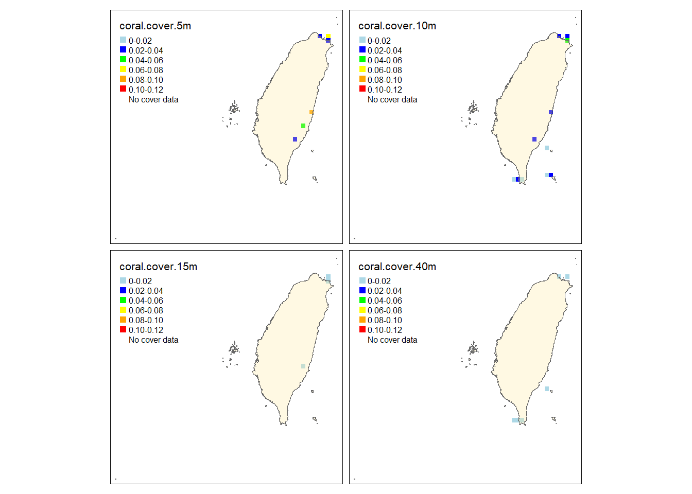
The observed and predicted maps are almost identical except that the coral cover at 5 and 10 meters in the east and the north are slightly different. Both of them show that S. pistillata has higher cover in the east and the north of Taiwan while the south have less cover. Also, the cover is higher at 5 and 10 meters.
Let’s also draw the predicted map for all the waters around Taiwan.
# grid with coral cover prediction
pred.5.map <- pred.5 ; pred.10.map <- pred.10
pred.15.map <- pred.15 ; pred.40.map <- pred.40
pred.5.map[is.na(pred.5.map)] <- 1 # replace the na with 1
pred.10.map[is.na(pred.10.map)] <- 1
pred.15.map[is.na(pred.15.map)] <- 1
pred.40.map[is.na(pred.40.map)] <- 1
sp.grd.pred.without <- SpatialGridDataFrame(grd,data=data.frame(Predicted.coral.cover.at.5m = pred.5.map, # create a spatial data frame with the predicted cover of all grids for mapping
                                                                Predicted.coral.cover.at.10m = pred.10.map,
                                                                Predicted.coral.cover.at.15m = pred.15.map,
                                                                Predicted.coral.cover.at.40m = pred.40.map),
                                            proj4string='+proj=longlat +datum=WGS84 +no_defs')
sp.grd.pred.without.sf <- st_as_sf(sp.grd.pred.without) # tranform the sp file to the sf file
# draw the maps for the predicted coral cover around Taiwan
tm_shape(sp.grd.pred.without.sf) +
  tm_symbols(c("Predicted.coral.cover.at.5m","Predicted.coral.cover.at.10m", "Predicted.coral.cover.at.15m","Predicted.coral.cover.at.40m"),
             size=1,breaks = c(seq(0,0.12,0.02),1),
             palette = col.pan, title.size = 5,border.col =NA,shape=15,
             labels = c("0-0.02", "0.02-0.04", "0.04-0.06","0.06-0.8","0.08-0.10","0.10-0.12","Missing data")) +
tm_shape(taiwan.sf) +
  tm_polygons("Islands",legend.show = F,alpha =.3)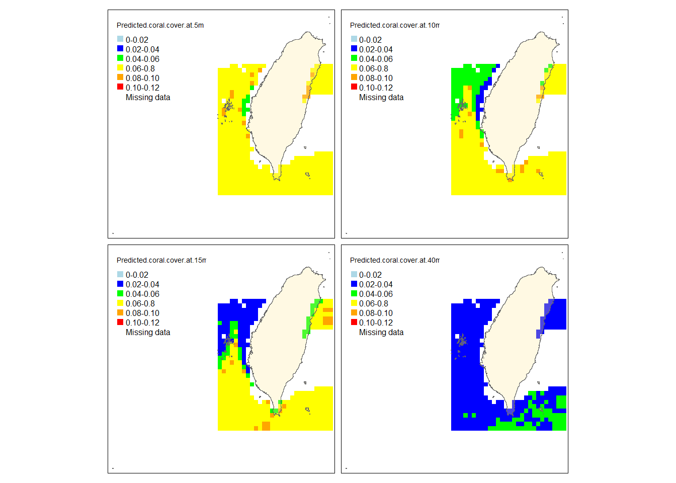
This predicted map shows that the cover of S. pistillata strongly decrease when approaching to the deeper depth. The cover in the western waters is generally less than that in the south except that more cover can be found in some areas of the western waters at 5 meters. The missing data mainly concentrate in the eastern and northern waters. Note that this prediction is based on the three environmental factors only, the real bathymetry is not considered here.
Based on the distribution maps and the RF model, we can deduce that S. pistillata tends to live in the water with higher light intensity and lower SST, mainly concentrating at shallow waters in the north and east. The deduction for the light makes sense because this coral species needs light to support the growth of their zooxanthellate, which can in turn provide the coral species energy. They, therefore, have more chance to appear at shallower depth (<15 meters). Despite tropical scleractinian corals usually favor warm and bright areas, S. pistillata is more abundant in the north and east where the SST is lower. This might be because this species is not competitive enough to other coral species when the thermal environment is suitable for growth, so they are not abundant in the south where the thermal condition can allow many coral species to develop. However, there is another possibility that this dataset may suffer from oversampling in the shallower water of the north (26% of the transects sampled at < 20 meters in the north, 19% of the transects sampled at < 20 meters in the east, 17% of the transects sampled at < 20 meters in the Orchid Island, Green Island and Kenting are less than 17%). It may make the algorithm have more chances to sample the transects in the north when bootstrapping, hence, the results would bias toward the environment of the north shallow water where is colder and lighter. More sampling effort needs to be added to the areas other than the shallow water in the north of Taiwan to make sure if this can be an issue or not.
Overall, this RF model suggests that the all abiotic variables (SST, light at the surveyed depth, and chlorophyll a) positively contribute to the cover of S. pistillata. Among these variables, the light is the strongest predictor. With these three factors, we can already catch 25.43% of the total variance. Nonetheless, considering the number of observations and also the number of variables, this dataset is too small to build a very robust RF model. Further sample effort is needed to make this prediction stronger especially in places other than the shallow water in the north of Taiwan.
Summary
RF can integrate different types of variables as well as a large amount of data, and seek for the complex relationship between the predicted variables and the response variables that sometimes the linear-based model cannot find. These features allow RF to stand out as one of the most popular approaches in modeling species distribution, in which the complex and dependent relationship commonly exists within and among environmental factors. Furthermore, based on a robust RF model, a prediction on the future alteration of species distribution considering the human-driven changes in any environmental parameters can be further estimated. This information could be quite helpful in conservation.
Reference
Bruno JF, Stachowicz JJ, Bertness MD (2003) Inclusion of facilitation into ecological theory. Trends in Ecology and Evolution 18:119-125
Busby JR (1991) BIOCLIM – a bioclimate analysis and prediction system. pp. 64–68 in Margules, C.R. and Austin, M.P. (eds). Nature conservation: cost effective Bbiological surveys and data analysis. CSIRO: Melbourne
Cutler DR, Edwards TC, Beard KH, Catler A, Hess KT, Gibson J, Lawler JJ (2007) Random forest for classification in ecology. Ecology 88:2783–2792
Elton CS (1927) Animal ecology. Sedgwick & Jackson, London, U.K
Grinnell J (1917) The niche-relationships of the California trasher. The Auk 34:427-433
Hutchinson GE (1957) Concluding remarks, cold spring harbor symposium. Quantitative Biology 22:415-427
Jeffrey S. Evans, Melanie A. Murphy, Zachary A. Holden, Cushman SA (2011) Modeling species distribution and change using random forest. In: Drew CA, Wiersma YF, Huettmann F (eds) Predictive species and habitat modeling in landscape ecology. Springer New York Dordrecht Heidelberg London
Johnson RH (1910) Determinate evolution in the color-pattern of the lady-beetles. Carnegie Inst. of Washington, Washington, D.C., USA
Phillips SJ, Anderson RP, Schapire RP (2006) Maximum entropy modeling of species geographic distributions. Ecological Modelling, 190: 231–259
Soberon J (2007) Grinnellian and Eltonian niches and geographic distributions of species. Ecology Letter 10:1115-1123 [10.1111/j.1461-0248.2007.01107.x]
https://builtin.com/data-science/random-forest-algorithm
https://towardsdatascience.com/understanding-random-forest-58381e0602d2
https://damariszurell.github.io/SDM-Intro/#1_Background
© Copyright 2022 Yuting Vicky Lin